
Median
Understanding the concept of the median, its uses and limitations
Last updated on 2 November 2026
Understanding median
The median is the “middle value” in a data set after all values have been arranged in ascending order, from smallest to largest.
At least half of the values are equal to or smaller than the median, while at least half are equal to or greater than the median. The median therefore separates the lower half of the values from the upper half.
How to find the median
Step 1: Arrange the values in ascending order
Given a set of data, such as wages, arrange the values from smallest to largest.
For example, suppose five employees earn the following monthly wages:
Person A: $1,800
Person B: $9,000
Person C: $5,000
Person D: $3,400
Person E: $6,000
When arranged in ascending order, the wages are:
$1,800 → $3,400 → $5,000 → $6,000 → $9,000

Step 2: Find the middle value
If the number of observations is odd, the number in the middle of the list is the median. This can be found by taking the value of the (n + 1) ÷ 2-th observation, where n is the number of observations.
If there is an even number of values, the median is the simple average of the two values in the middle. These are the n ÷ 2-th and (n ÷ 2 + 1)-th observations.
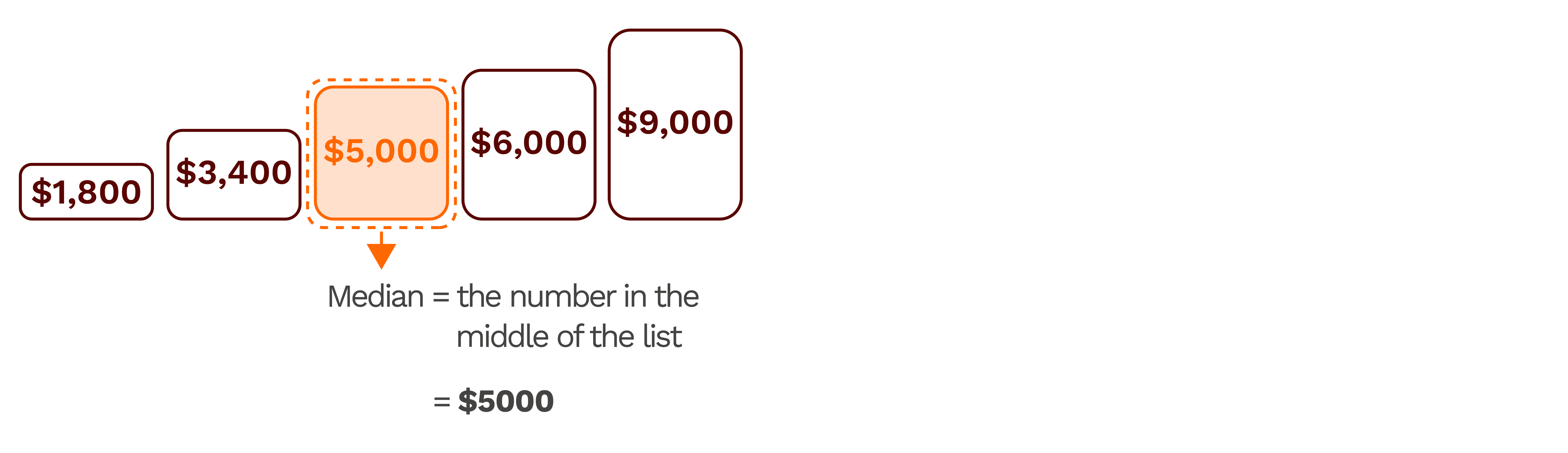
As there are five observations (i.e. odd number), the median is Person C's wages.
Example 1: Odd Number of Observations
Suppose Middle World Co. would like to compare its employees' age profile with that of other companies in the industry.
Table of the ages of Middle World Co.'s nine employees, arranged from youngest to oldest.
S/N | Name | Age (years) |
1 | Timmy | 17 |
2 | Lorna | 20 |
3 | Simien | 43 |
4 | Tammy | 45 |
5 | Lucius | 50 |
6 | Jane | 53 |
7 | Simon | 55 |
8 | Marla | 59 |
9 | Ray | 62 |
Question: What is the median age of these nine employees?
Solution: Since there is an odd number of observations and the ages are arranged from youngest to oldest, the median is the age of the employee in the middle.
The position of the median is:
(n + 1) ÷ 2 = (9 + 1) ÷ 2 = 5th observation
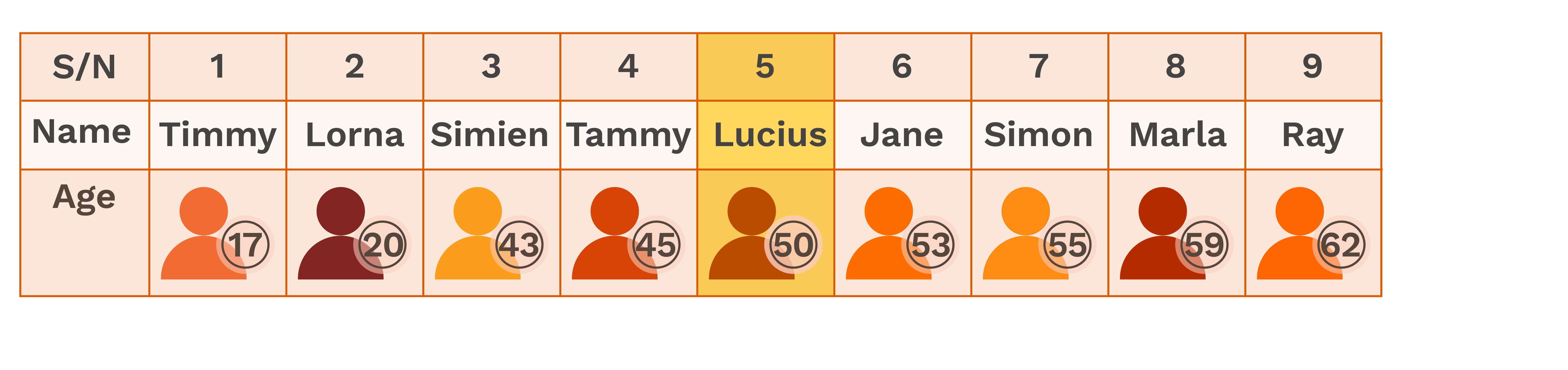
The fifth employee is Lucius, who is 50 years old. Therefore, the median age is 50 years.
*Note that if Middle World does not hire new workers and no workers leave, Lucius’s age will always be the median age, no matter how many years have passed.
Example 2: Even Number of Observations
Suppose we have the monthly wages of ten employees in a company. Their wages are arranged below from lowest to highest.
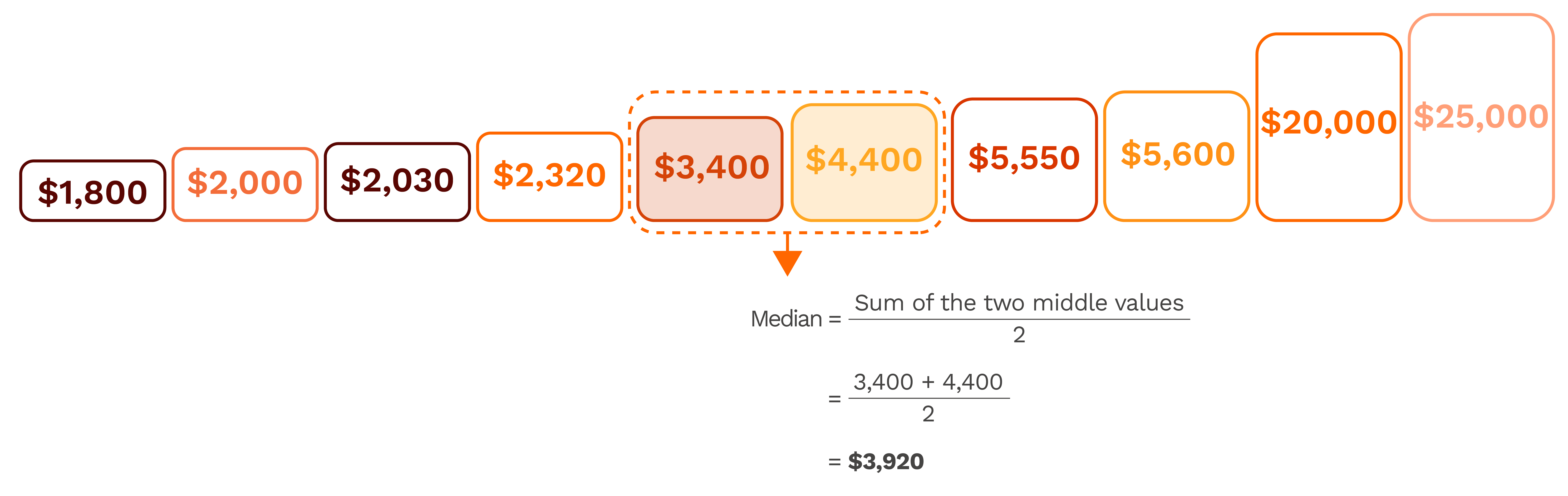
Since there are ten observations, which is an even number, the median is the simple average of the fifth and sixth observations.
The fifth and sixth wages are $3,400 and $4,440.
Therefore:
Median = ($3,400 + $4,440) ÷ 2
= $3,920
The median monthly wage is $3,920.
Uses of the median
The median can be used to represent the typical value of a data set. It is particularly useful when the data contains extreme values.
When to use the median instead of the mean
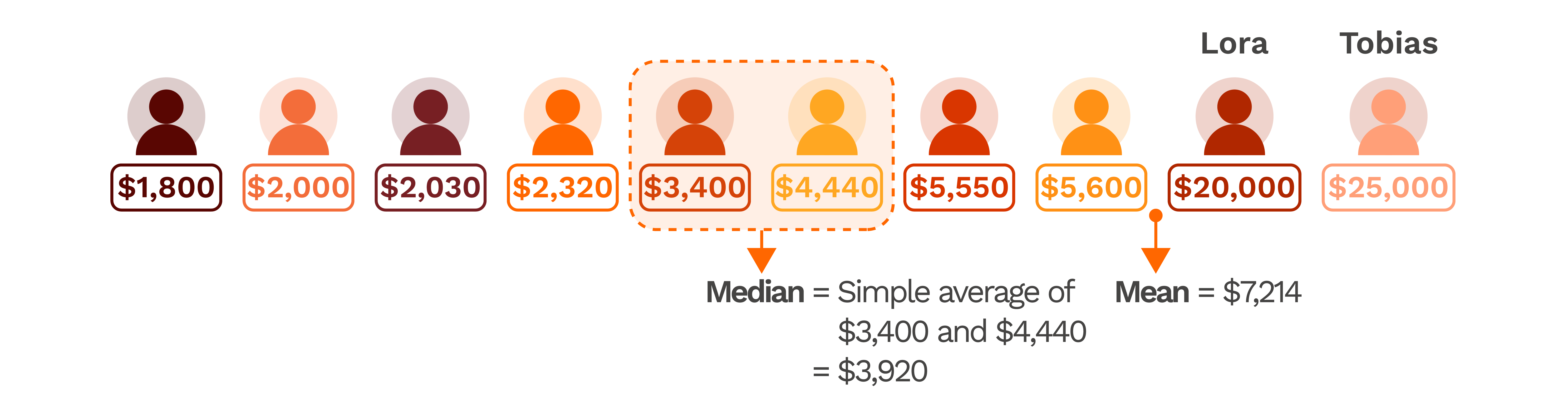
Using the wages of the ten employees in the previous example, the median monthly wage is $3,920, while the mean (i.e. average) monthly wage is $7,214.
The mean is much higher than the median because Lora and Tobias earn $20,000 and $25,000 respectively, which are much higher than the wages of the other employees.
As the mean takes every value into account, these extreme values pull the average upwards, making the mean greater. The median, on the other hand, is determined by the middle values and is not affected by the size of these extreme values.
In this example, the median therefore provides a better representation of the typical wage.
Limitations
While the median is less affected by extreme values, it does not take into account the size of every value in the data set.
For example, suppose Lora and Tobias now earn $6,000 each instead of $20,000 and $25,000 respectively.
The median remains at $3,920, while the mean becomes $3,914.
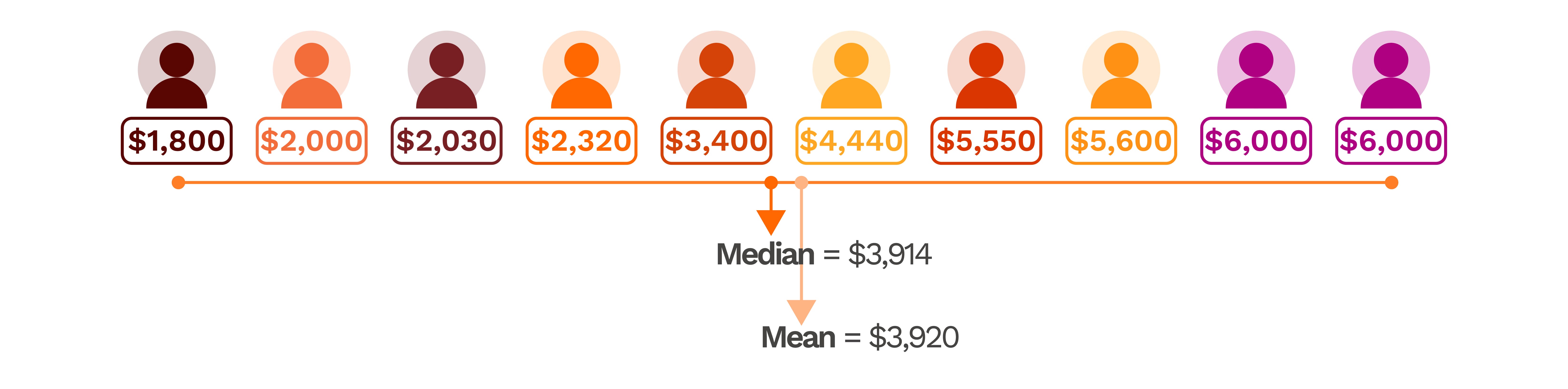
When there are no extreme values that significantly affect the data, the mean may provide a better summary because it takes every observation into account, rather than only the middle value or values.
As the mean takes all values into account, it can also be used for further calculations. For example, the total income paid by an employer can be derived when the mean income and number of employees are known – by multiplying the mean income by number of employees.
Using the mean and median to determine skewness
Distribution describes how the values in a dataset are spread out. It shows which values are common, which are less common, and the overall shape of the data.
For example, if we look at workers' monthly salaries, the distribution tells us how salaries are spread across workers – from lower to higher salaries.
Skewness describes whether a distribution is asymmetric, meaning that the values are more spread out on one side than the other.
When the mean and median are similar, the distribution is likely to be roughly symmetric.
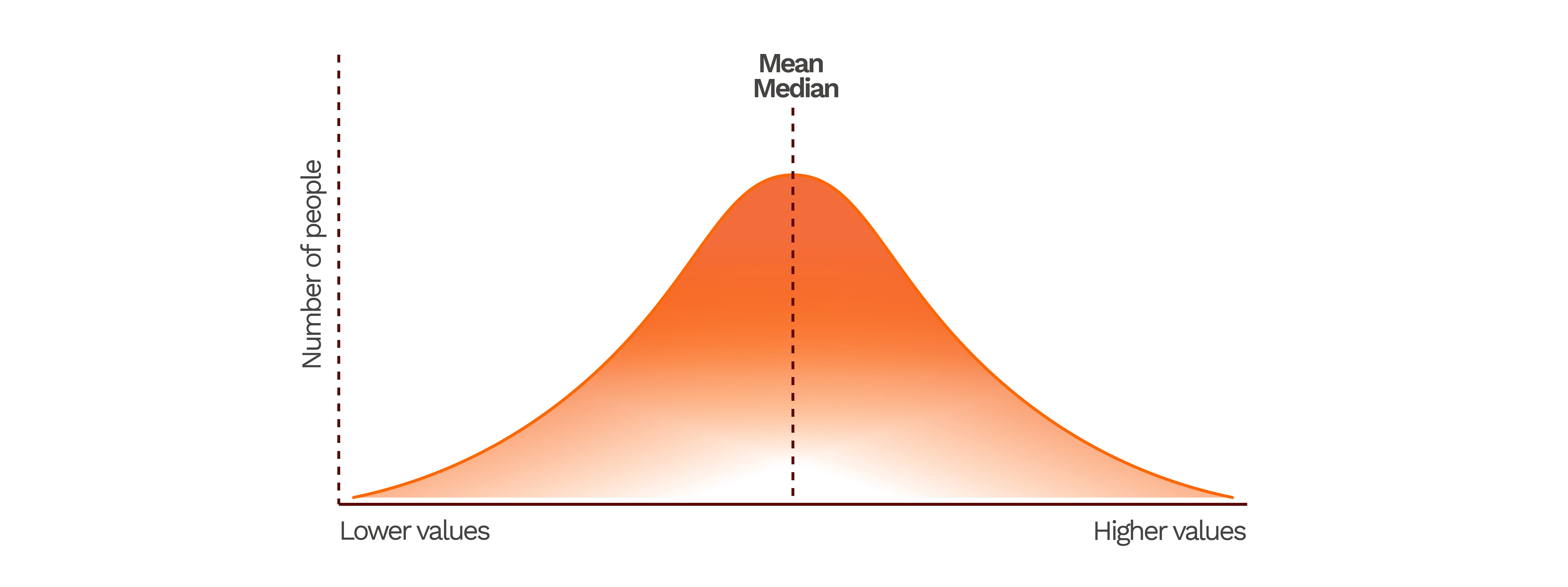
When the mean is higher than the median, relatively high values pull the mean upwards, suggesting that the distribution is positively (right) skewed.
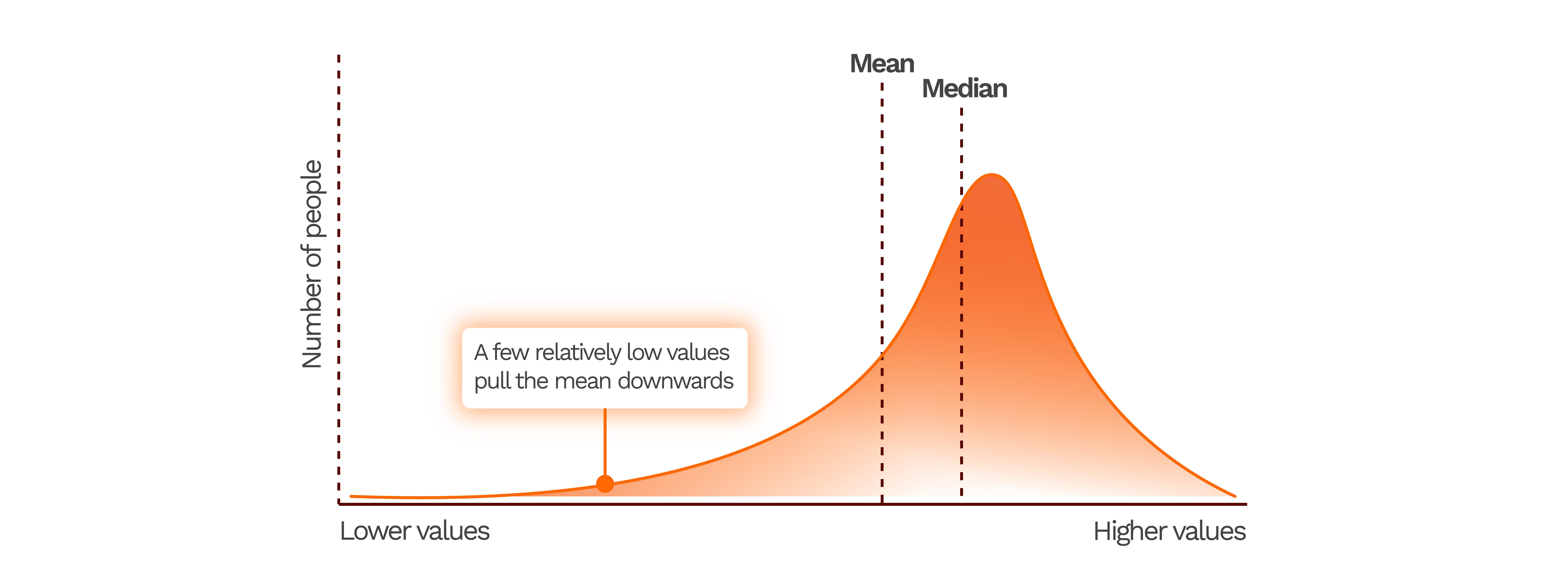
When the mean is lower than the median, relatively low values pull the mean downwards, suggesting that the distribution is negatively (left) skewed.
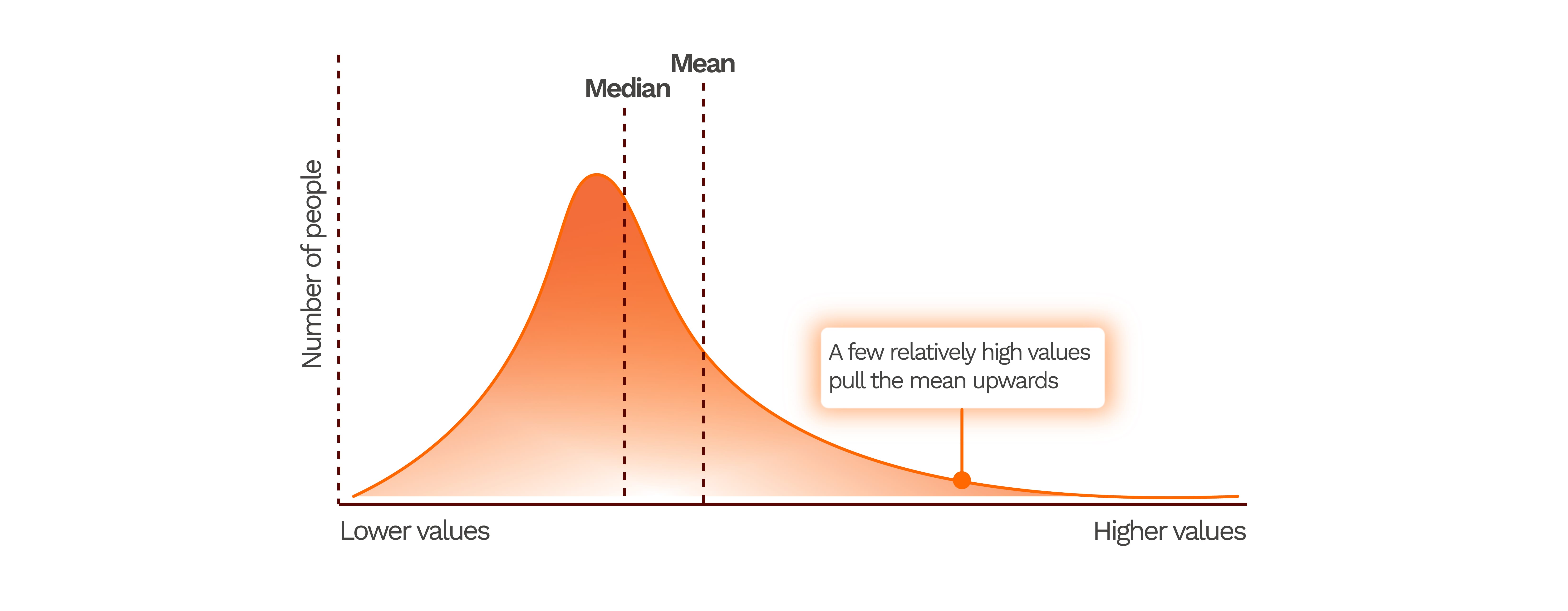
Hence, the greater the difference between the mean and median, the stronger the indication that the distribution may be skewed. However, comparing the mean and median provides only an indication of skewness and does not by itself determine the exact shape or degree of skewness.