
Seasonal Adjustment
Understanding the concept of seasonal adjustment, its uses and limitations
Last updated on 1 November 2026
Understanding seasonal adjustment
In analysing labour market statistics, we are often interested in understanding how the indicator has changed over time, for example compared with the previous quarter or the same period last year.
Time Series
A time series refers to a sequence of observations on a specific variable, collected over periodic time intervals, e.g. a day, week, month, quarter, or year.
Examples:
Number of persons in the labour force in June each year
Change in employment in each quarter
Number of job vacancies at the end of each quarter
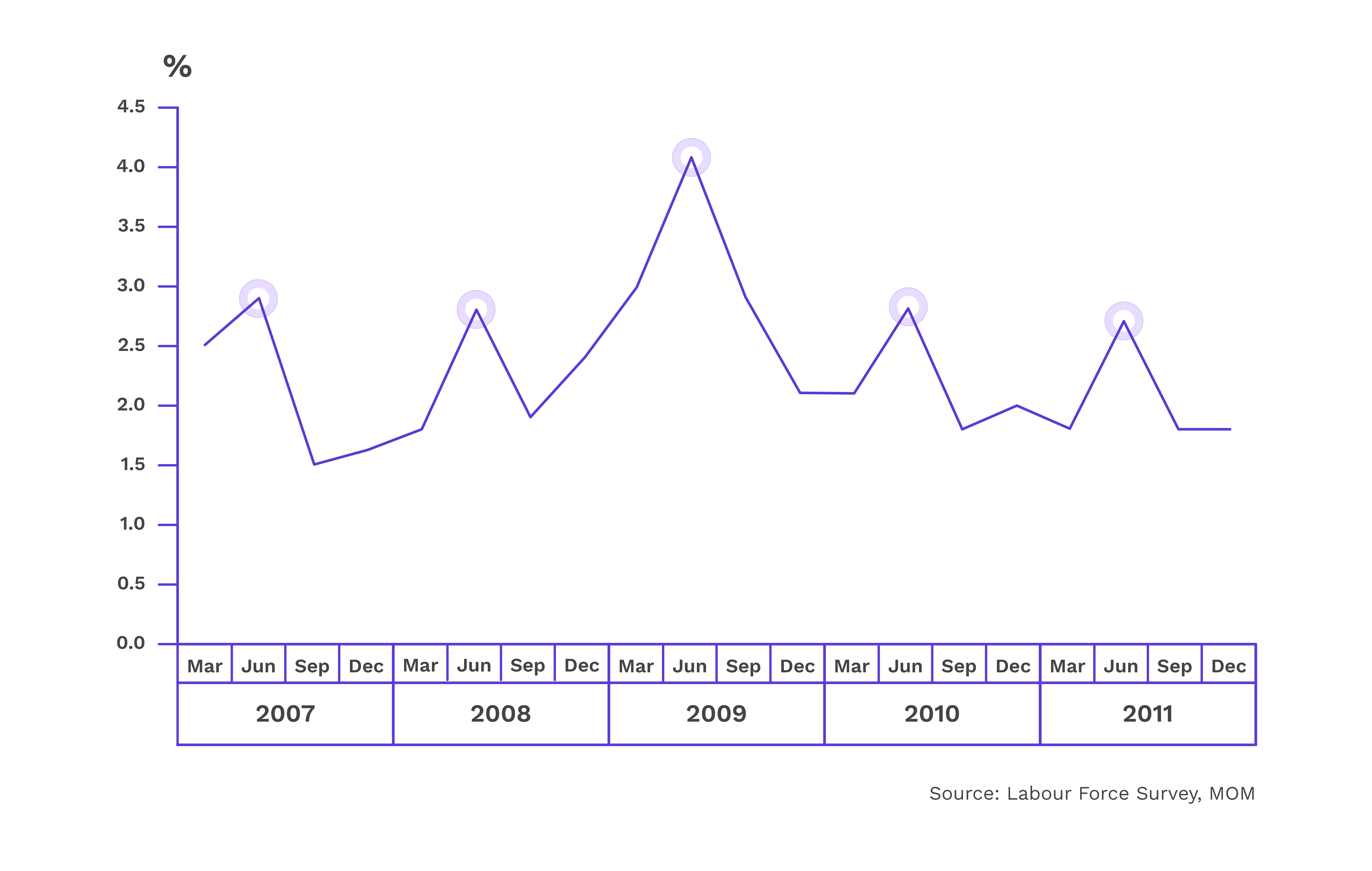
Overall unemployment rate measured at quarterly intervals (refer to chart in Example 1)
Seasonality
Seasonality refers to the periodic variation in a time series that repeats in the same period each year.
Example 1
The unemployment rate typically increases form March to June and decreases from June to September. Unemployment is typically higher in June, when final year students from universities look for jobs, and seek vacation jobs during their mid-year break.
Overall Unemployment Rate (Non-Seasonally Adjusted)
Example 2
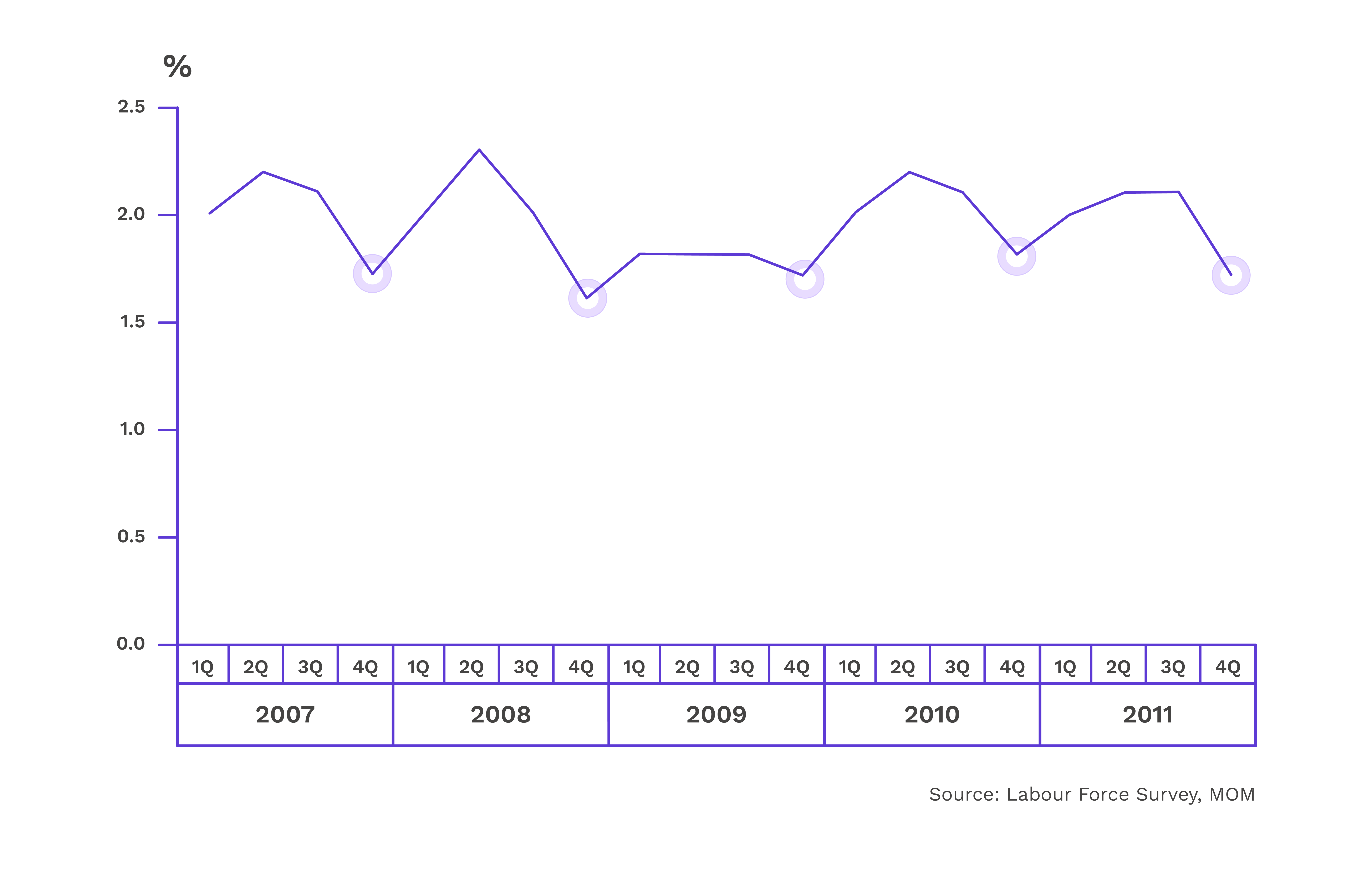
Resignation rate is typically lower in the last quarter of the year (i.e. October to December). Given that year-end bonuses are typically paid out during this time of the year, employees who intend to change jobs may decide to stay on and receive their bonus first, before moving to a new job.
Average Monthly Resignation Rate (Non-Seasonally Adjusted)
If a time series periodically increases (or decreases) at same periods during the year, it will be difficult for us to analyse whether the changes in the indicator are a true reflection of economic or labour market conditions or merely due to seasonal influences.
To better discern the trend (or long-term movement of the variable) and cyclical patterns (a component of the series that changes with the economic cycle) in the time series, many national statistical agencies apply a statistical technique known as seasonal adjustment to the time series to remove the seasonal influences.
This can be done using statistical software with seasonal adjustment functionality. Time series with seasonal influences removed are called seasonally adjusted series.
Uses of seasonal adjustment
Seasonal adjustment helps us make a more meaningful analysis of the trends in a data series, especially for those with strong seasonal patterns.
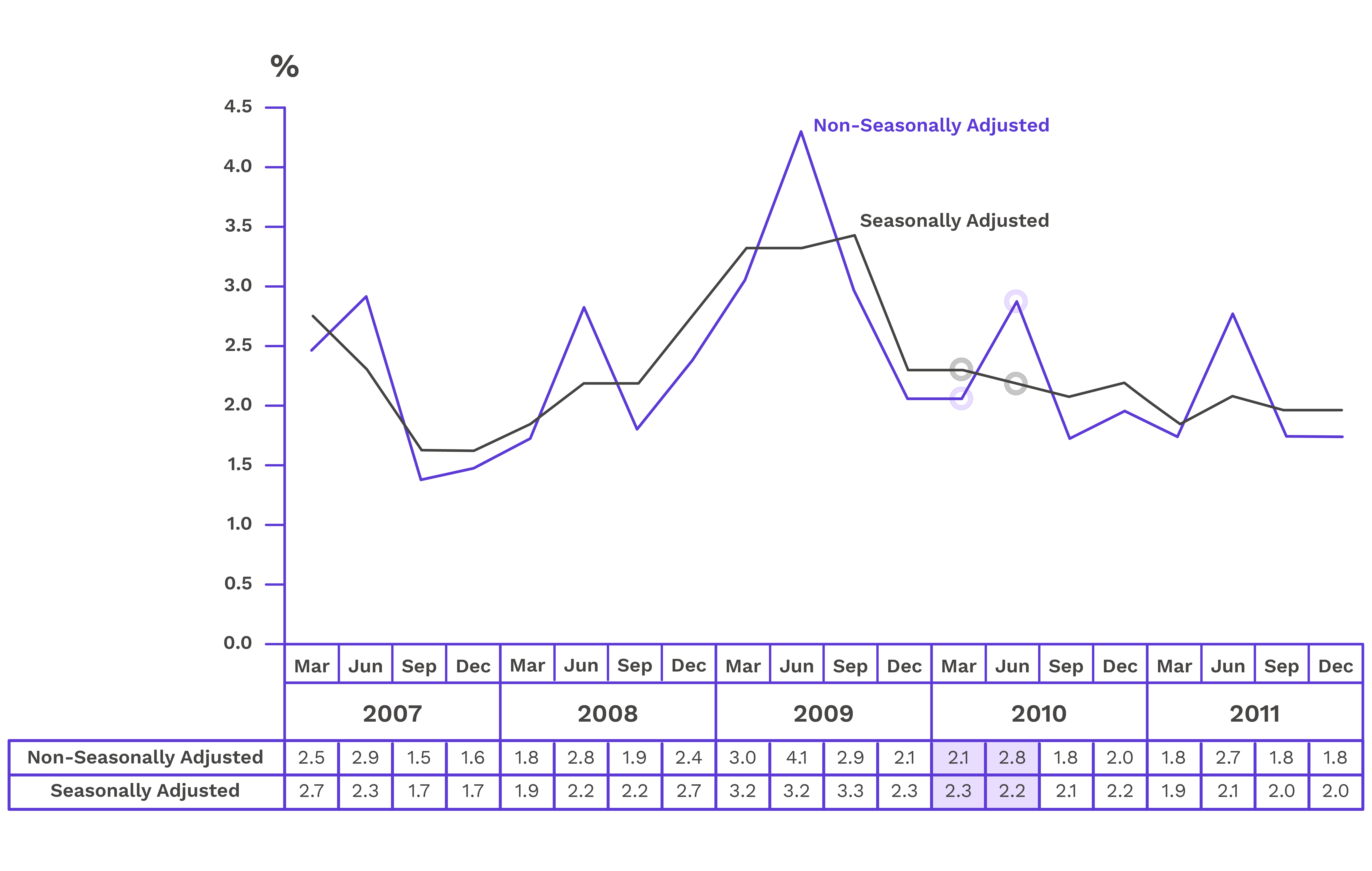
For example, consider the unemployment rate data in the following chart. As unemployment rate is usually high in June, it is difficult to ascertain if the increase in non-seasonally adjusted unemployment rate from 2.1% in March 2010 to 2.8% in June 2010 was a reflection of economic conditions or due to seasonal factors.
After removing the seasonal component from the data series, we see that the seasonally adjusted unemployment rate had in fact declined from 2.3% in March 2010 to 2.2% in June 2010, suggesting that the underlying unemployment situation was broadly stable.
Overall Unemployment Rate
Note: The seasonally adjusted unemployment figures are subject to annual revisions when the latest set of seasonal factors is updated, taking into account observations for the latest available year. The most up-to-date data can be accessed here.
Limitations
For indicators with strong seasonal patterns, comparisons between consecutive periods (e.g. quarters) should not be done using non-seasonally adjusted series.
Referring to the chart for Overall Unemployment Rate above, a person looking at the time series of the non-seasonally adjusted unemployment rate may come to the conclusion that unemployment had worsened in June 2010 compared with March 2010, on the basis that the rate increased from 2.1% to 2.8%.
It turned out that the unemployment rate was actually slightly lower in June 2010 compared with March 2010, after we remove the seasonal component from the time series.
In analysing time series data especially those that display strong seasonal patterns, it would be more appropriate to consider the quarter-on-quarter or month-on-month changes based on the seasonally adjusted data. This allows for a more meaningful comparison of the time series trends rather than that based on the non-seasonally adjusted series, as changes in the unadjusted data over the quarter or over the month due to seasonal influences may mistakenly be taken as a change due to trend or cyclical factors.
In the absence of seasonally adjusted data for a time series, it would be more meaningful to study the changes in the time series compared with the same period of each year. The exception is for series which do not have identifiable seasonal patterns, or where the seasonal patterns are weak.
For example, we want to study the trends in the unemployment rate for a group where seasonally adjusted data is not available. In this case, we should compare the changes between the same period across years (e.g. unemployment rate in June this year, compared with unemployment rate in June last year and/or in earlier years). This would allow us to make a better assessment of the trends in the data without it being distorted by seasonal patterns. Alternatively, for a comparison across years, we could use the annual average, which provides a measure of the indicator for the whole year.
Note also that seasonally adjusted data are not comparable with non-seasonally adjusted data. For example, one should not compare the seasonally adjusted resignation rate for the fourth quarter of 2011 with the non-seasonally adjusted resignation rate in the third quarter of 2011, and conclude that the resignation rate has increased, decreased or stayed the same.